Demo for the DoWhy causal API

We show a simple example of adding a causal extension to any dataframe.

import dowhy.datasets
import dowhy.api

import numpy as np
import pandas as pd

from statsmodels.api import OLS

data = dowhy.datasets.linear_dataset(beta=5,
        num_common_causes=1,
        num_instruments = 0,
        num_samples=1000,
        treatment_is_binary=True)
df = data['df']
df['y'] = df['y'] + np.random.normal(size=len(df)) # Adding noise to data. Without noise, the variance in Y|X, Z is zero, and mcmc fails.
#data['dot_graph'] = 'digraph { v ->y;X0-> v;X0-> y;}'

treatment= data["treatment_name"][0]
outcome = data["outcome_name"][0]
common_cause = data["common_causes_names"][0]
df

	W0	v0	y
0	0.076236	True	5.553473
1	0.060844	False	0.368952
2	-0.028633	False	-0.494726
3	-1.427719	True	5.404953
4	-0.671959	False	-1.001133
...	...	...	...
995	0.700718	True	5.251570
996	0.946380	True	7.180262
997	-0.004310	True	4.482246
998	0.618509	True	4.455502
999	-1.381954	False	-0.086505

1000 rows × 3 columns

# data['df'] is just a regular pandas.DataFrame
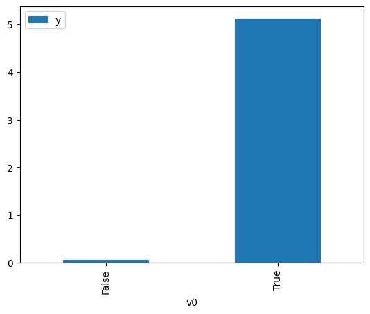
df.causal.do(x=treatment,
                     variable_types={treatment: 'b', outcome: 'c', common_cause: 'c'},
                     outcome=outcome,
                     common_causes=[common_cause],
                     proceed_when_unidentifiable=True).groupby(treatment).mean().plot(y=outcome, kind='bar')

<AxesSubplot: xlabel='v0'>

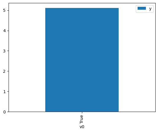
df.causal.do(x={treatment: 1},
              variable_types={treatment:'b', outcome: 'c', common_cause: 'c'},
              outcome=outcome,
              method='weighting',
              common_causes=[common_cause],
              proceed_when_unidentifiable=True).groupby(treatment).mean().plot(y=outcome, kind='bar')

<AxesSubplot: xlabel='v0'>

cdf_1 = df.causal.do(x={treatment: 1},
              variable_types={treatment: 'b', outcome: 'c', common_cause: 'c'},
              outcome=outcome,
              dot_graph=data['dot_graph'],
              proceed_when_unidentifiable=True)

cdf_0 = df.causal.do(x={treatment: 0},
              variable_types={treatment: 'b', outcome: 'c', common_cause: 'c'},
              outcome=outcome,
              dot_graph=data['dot_graph'],
              proceed_when_unidentifiable=True)

cdf_0

	W0	v0	y	propensity_score	weight
0	-0.352919	False	0.446923	0.584806	1.709968
1	0.814069	False	0.333252	0.282563	3.539036
2	-2.343394	False	1.050524	0.925262	1.080776
3	0.828998	False	-0.382004	0.279270	3.580766
4	1.064405	False	0.701340	0.230561	4.337242
...	...	...	...	...	...
995	0.895503	False	0.163814	0.264889	3.775160
996	2.014276	False	-0.379485	0.096009	10.415706
997	-0.376085	False	-0.769199	0.590935	1.692233
998	1.836714	False	1.371098	0.114205	8.756149
999	0.428957	False	-0.634386	0.374900	2.667378

1000 rows × 5 columns

cdf_1

	W0	v0	y	propensity_score	weight
0	1.303760	True	5.675314	0.812527	1.230728
1	1.436695	True	6.111159	0.833644	1.199553
2	0.631619	True	6.052427	0.675366	1.480680
3	0.354007	True	6.152660	0.605733	1.650893
4	-2.741986	True	2.913577	0.049674	20.131449
...	...	...	...	...	...
995	0.721921	True	5.594780	0.696601	1.435543
996	1.337709	True	3.280717	0.818109	1.222331
997	-2.741986	True	2.913577	0.049674	20.131449
998	1.812561	True	5.540571	0.883099	1.132376
999	0.124867	True	5.605328	0.544679	1.835943

1000 rows × 5 columns

Comparing the estimate to Linear Regression

First, estimating the effect using the causal data frame, and the 95% confidence interval.

(cdf_1['y'] - cdf_0['y']).mean()

$\displaystyle 5.06489946748145$

1.96*(cdf_1['y'] - cdf_0['y']).std() / np.sqrt(len(df))

$\displaystyle 0.0887509312439617$

Comparing to the estimate from OLS.

model = OLS(np.asarray(df[outcome]), np.asarray(df[[common_cause, treatment]], dtype=np.float64))
result = model.fit()
result.summary()

OLS Regression Results

Dep. Variable:	y	R-squared (uncentered):	0.942
Model:	OLS	Adj. R-squared (uncentered):	0.941
Method:	Least Squares	F-statistic:	8038.
Date:	Fri, 16 Dec 2022	Prob (F-statistic):	0.00
Time:	19:37:21	Log-Likelihood:	-1410.4
No. Observations:	1000	AIC:	2825.
Df Residuals:	998	BIC:	2835.
Df Model:	2
Covariance Type:	nonrobust

	coef	std err	t	P>|t|	[0.025	0.975]
x1	0.2405	0.036	6.761	0.000	0.171	0.310
x2	5.0122	0.048	104.315	0.000	4.918	5.106

Omnibus:	1.561	Durbin-Watson:	1.932
Prob(Omnibus):	0.458	Jarque-Bera (JB):	1.428
Skew:	-0.062	Prob(JB):	0.490
Kurtosis:	3.137	Cond. No.	1.94

Notes:
[1] R² is computed without centering (uncentered) since the model does not contain a constant.
[2] Standard Errors assume that the covariance matrix of the errors is correctly specified.