Conditional Average Treatment Effects (CATE) with DoWhy and EconML
This is an experimental feature where we use EconML methods from DoWhy. Using EconML allows CATE estimation using different methods.
All four steps of causal inference in DoWhy remain the same: model, identify, estimate, and refute. The key difference is that we now call econml methods in the estimation step. There is also a simpler example using linear regression to understand the intuition behind CATE estimators.
All datasets are generated using linear structural equations.
[1]:
%load_ext autoreload
%autoreload 2
[2]:
import numpy as np
import pandas as pd
import logging

import dowhy
from dowhy import CausalModel
import dowhy.datasets

import econml
import warnings
warnings.filterwarnings('ignore')

BETA = 10
[3]:
data = dowhy.datasets.linear_dataset(BETA, num_common_causes=4, num_samples=10000,
                                    num_instruments=2, num_effect_modifiers=2,
                                     num_treatments=1,
                                    treatment_is_binary=False,
                                    num_discrete_common_causes=2,
                                    num_discrete_effect_modifiers=0,
                                    one_hot_encode=False)
df=data['df']
print(df.head())
print("True causal estimate is", data["ate"])
         X0        X1   Z0        Z1        W0        W1 W2 W3         v0  \
0  0.184316  1.023765  0.0  0.746975 -1.064751 -1.655496  0  2   4.303728
1 -0.098788 -0.271350  0.0  0.056506  0.685865  0.745997  2  3  11.380914
2 -1.430053 -0.788282  0.0  0.102457 -0.513976 -0.473495  3  1   7.679942
3  0.164521 -1.147925  0.0  0.054876 -0.759346 -0.197663  0  1  -0.192062
4  0.248026 -0.251351  1.0  0.447742 -1.551764 -2.543249  3  3  16.796109

            y
0   51.187076
1  120.013064
2   39.207876
3   -1.783893
4  173.186709
True causal estimate is 9.628211731869985
[4]:
model = CausalModel(data=data["df"],
                    treatment=data["treatment_name"], outcome=data["outcome_name"],
                    graph=data["gml_graph"])
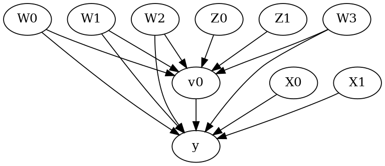
[5]:
model.view_model()
from IPython.display import Image, display
display(Image(filename="causal_model.png"))
[6]:
identified_estimand= model.identify_effect(proceed_when_unidentifiable=True)
print(identified_estimand)
Estimand type: EstimandType.NONPARAMETRIC_ATE

### Estimand : 1
Estimand name: backdoor
Estimand expression:
  d
─────(E[y|W1,W0,W2,W3])
d[v₀]
Estimand assumption 1, Unconfoundedness: If U→{v0} and U→y then P(y|v0,W1,W0,W2,W3,U) = P(y|v0,W1,W0,W2,W3)

### Estimand : 2
Estimand name: iv
Estimand expression:
 ⎡                              -1⎤
 ⎢    d        ⎛    d          ⎞  ⎥
E⎢─────────(y)⋅⎜─────────([v₀])⎟  ⎥
 ⎣d[Z₀  Z₁]    ⎝d[Z₀  Z₁]      ⎠  ⎦
Estimand assumption 1, As-if-random: If U→→y then ¬(U →→{Z0,Z1})
Estimand assumption 2, Exclusion: If we remove {Z0,Z1}→{v0}, then ¬({Z0,Z1}→y)

### Estimand : 3
Estimand name: frontdoor
No such variable(s) found!
Linear Model
First, let us build some intuition using a linear model for estimating CATE. The effect modifiers (that lead to a heterogeneous treatment effect) can be modeled as interaction terms with the treatment. Thus, their value modulates the effect of treatment.
Below the estimated effect of changing treatment from 0 to 1.
[7]:
linear_estimate = model.estimate_effect(identified_estimand,
                                        method_name="backdoor.linear_regression",
                                       control_value=0,
                                       treatment_value=1)
print(linear_estimate)
*** Causal Estimate ***

## Identified estimand
Estimand type: EstimandType.NONPARAMETRIC_ATE

### Estimand : 1
Estimand name: backdoor
Estimand expression:
  d
─────(E[y|W1,W0,W2,W3])
d[v₀]
Estimand assumption 1, Unconfoundedness: If U→{v0} and U→y then P(y|v0,W1,W0,W2,W3,U) = P(y|v0,W1,W0,W2,W3)

## Realized estimand
b: y~v0+W1+W0+W2+W3+v0*X0+v0*X1
Target units: ate

## Estimate
Mean value: 9.628235916738104
EconML methods
We now move to the more advanced methods from the EconML package for estimating CATE.
First, let us look at the double machine learning estimator. Method_name corresponds to the fully qualified name of the class that we want to use. For double ML, it is “econml.dml.DML”.
Target units defines the units over which the causal estimate is to be computed. This can be a lambda function filter on the original dataframe, a new Pandas dataframe, or a string corresponding to the three main kinds of target units (“ate”, “att” and “atc”). Below we show an example of a lambda function.
Method_params are passed directly to EconML. For details on allowed parameters, refer to the EconML documentation.
[8]:
from sklearn.preprocessing import PolynomialFeatures
from sklearn.linear_model import LassoCV
from sklearn.ensemble import GradientBoostingRegressor
dml_estimate = model.estimate_effect(identified_estimand, method_name="backdoor.econml.dml.DML",
                                     control_value = 0,
                                     treatment_value = 1,
                                 target_units = lambda df: df["X0"]>1,  # condition used for CATE
                                 confidence_intervals=False,
                                method_params={"init_params":{'model_y':GradientBoostingRegressor(),
                                                              'model_t': GradientBoostingRegressor(),
                                                              "model_final":LassoCV(fit_intercept=False),
                                                              'featurizer':PolynomialFeatures(degree=1, include_bias=False)},
                                               "fit_params":{}})
print(dml_estimate)
*** Causal Estimate ***

## Identified estimand
Estimand type: EstimandType.NONPARAMETRIC_ATE

### Estimand : 1
Estimand name: backdoor
Estimand expression:
  d
─────(E[y|W1,W0,W2,W3])
d[v₀]
Estimand assumption 1, Unconfoundedness: If U→{v0} and U→y then P(y|v0,W1,W0,W2,W3,U) = P(y|v0,W1,W0,W2,W3)

## Realized estimand
b: y~v0+W1+W0+W2+W3 | X0,X1
Target units: Data subset defined by a function

## Estimate
Mean value: 14.495131695143286
Effect estimates: [[13.77887095]
 [13.75726448]
 [12.51609202]
 ...
 [14.57703812]
 [10.56353472]
 [11.59317826]]
[9]:
print("True causal estimate is", data["ate"])
True causal estimate is 9.628211731869985
[10]:
dml_estimate = model.estimate_effect(identified_estimand, method_name="backdoor.econml.dml.DML",
                                     control_value = 0,
                                     treatment_value = 1,
                                 target_units = 1,  # condition used for CATE
                                 confidence_intervals=False,
                                method_params={"init_params":{'model_y':GradientBoostingRegressor(),
                                                              'model_t': GradientBoostingRegressor(),
                                                              "model_final":LassoCV(fit_intercept=False),
                                                              'featurizer':PolynomialFeatures(degree=1, include_bias=True)},
                                               "fit_params":{}})
print(dml_estimate)
*** Causal Estimate ***

## Identified estimand
Estimand type: EstimandType.NONPARAMETRIC_ATE

### Estimand : 1
Estimand name: backdoor
Estimand expression:
  d
─────(E[y|W1,W0,W2,W3])
d[v₀]
Estimand assumption 1, Unconfoundedness: If U→{v0} and U→y then P(y|v0,W1,W0,W2,W3,U) = P(y|v0,W1,W0,W2,W3)

## Realized estimand
b: y~v0+W1+W0+W2+W3 | X0,X1
Target units:

## Estimate
Mean value: 9.566581240446085
Effect estimates: [[12.66641759]
 [ 9.06324629]
 [ 4.16475233]
 ...
 [10.75745638]
 [ 7.36737442]
 [ 8.17839377]]
CATE Object and Confidence Intervals
EconML provides its own methods to compute confidence intervals. Using BootstrapInference in the example below.
[11]:
from sklearn.preprocessing import PolynomialFeatures
from sklearn.linear_model import LassoCV
from sklearn.ensemble import GradientBoostingRegressor
from econml.inference import BootstrapInference
dml_estimate = model.estimate_effect(identified_estimand,
                                     method_name="backdoor.econml.dml.DML",
                                     target_units = "ate",
                                     confidence_intervals=True,
                                     method_params={"init_params":{'model_y':GradientBoostingRegressor(),
                                                              'model_t': GradientBoostingRegressor(),
                                                              "model_final": LassoCV(fit_intercept=False),
                                                              'featurizer':PolynomialFeatures(degree=1, include_bias=True)},
                                               "fit_params":{
                                                               'inference': BootstrapInference(n_bootstrap_samples=100, n_jobs=-1),
                                                            }
                                              })
print(dml_estimate)
*** Causal Estimate ***

## Identified estimand
Estimand type: EstimandType.NONPARAMETRIC_ATE

### Estimand : 1
Estimand name: backdoor
Estimand expression:
  d
─────(E[y|W1,W0,W2,W3])
d[v₀]
Estimand assumption 1, Unconfoundedness: If U→{v0} and U→y then P(y|v0,W1,W0,W2,W3,U) = P(y|v0,W1,W0,W2,W3)

## Realized estimand
b: y~v0+W1+W0+W2+W3 | X0,X1
Target units: ate

## Estimate
Mean value: 9.585337595143452
Effect estimates: [[12.71754568]
 [ 9.08152062]
 [ 4.08314366]
 ...
 [10.77288291]
 [ 7.33489019]
 [ 8.15373185]]
Can provide a new inputs as target units and estimate CATE on them.
[12]:
test_cols= data['effect_modifier_names'] # only need effect modifiers' values
test_arr = [np.random.uniform(0,1, 10) for _ in range(len(test_cols))] # all variables are sampled uniformly, sample of 10
test_df = pd.DataFrame(np.array(test_arr).transpose(), columns=test_cols)
dml_estimate = model.estimate_effect(identified_estimand,
                                     method_name="backdoor.econml.dml.DML",
                                     target_units = test_df,
                                     confidence_intervals=False,
                                     method_params={"init_params":{'model_y':GradientBoostingRegressor(),
                                                              'model_t': GradientBoostingRegressor(),
                                                              "model_final":LassoCV(),
                                                              'featurizer':PolynomialFeatures(degree=1, include_bias=True)},
                                               "fit_params":{}
                                              })
print(dml_estimate.cate_estimates)
[[12.51144473]
 [12.07468235]
 [11.1622291 ]
 [11.89897762]
 [12.95068227]
 [13.09547487]
 [13.62526954]
 [11.38264721]
 [13.01080906]
 [13.16179901]]
Can also retrieve the raw EconML estimator object for any further operations
[13]:
print(dml_estimate._estimator_object)
<econml.dml.dml.DML object at 0x7fb9ddadf610>
Works with any EconML method
In addition to double machine learning, below we example analyses using orthogonal forests, DRLearner (bug to fix), and neural network-based instrumental variables.
Binary treatment, Binary outcome
[14]:
data_binary = dowhy.datasets.linear_dataset(BETA, num_common_causes=4, num_samples=10000,
                                    num_instruments=2, num_effect_modifiers=2,
                                    treatment_is_binary=True, outcome_is_binary=True)
# convert boolean values to {0,1} numeric
data_binary['df'].v0 = data_binary['df'].v0.astype(int)
data_binary['df'].y = data_binary['df'].y.astype(int)
print(data_binary['df'])

model_binary = CausalModel(data=data_binary["df"],
                    treatment=data_binary["treatment_name"], outcome=data_binary["outcome_name"],
                    graph=data_binary["gml_graph"])
identified_estimand_binary = model_binary.identify_effect(proceed_when_unidentifiable=True)
            X0        X1   Z0        Z1        W0        W1        W2  \
0     1.407181 -1.006574  1.0  0.936970 -0.560792  3.675080  1.695422
1     0.788738  0.233188  0.0  0.611156 -0.255626  1.361288  1.077083
2     1.567530  0.521190  1.0  0.032971 -0.108569  2.273863  0.085113
3     0.352918 -0.840284  0.0  0.040884  0.007009  2.733734  0.281024
4     0.008780 -1.696901  0.0  0.180170 -1.088745  0.990502  1.812114
...        ...       ...  ...       ...       ...       ...       ...
9995 -0.142011  1.028627  0.0  0.957043 -1.500051  0.998575  0.511238
9996  0.851902  2.266624  0.0  0.678300 -0.701726  0.748294  1.628316
9997 -0.171566  0.033419  1.0  0.092534 -0.118482  0.253016 -0.289634
9998  0.537959 -0.200492  1.0  0.943669 -1.749916  0.629262  1.241166
9999  0.352818 -0.332338  1.0  0.523575 -1.927553 -0.576147  1.703810

            W3  v0  y
0     0.219969   1  1
1     0.415013   1  1
2    -2.174826   1  1
3    -1.356104   1  1
4    -0.820616   1  0
...        ...  .. ..
9995  0.658315   1  1
9996  1.337809   1  1
9997  0.114054   1  1
9998 -2.240528   1  0
9999  1.526971   1  1

[10000 rows x 10 columns]
Using DRLearner estimator
[15]:
from sklearn.linear_model import LogisticRegressionCV
#todo needs binary y
drlearner_estimate = model_binary.estimate_effect(identified_estimand_binary,
                                method_name="backdoor.econml.dr.LinearDRLearner",
                                confidence_intervals=False,
                                method_params={"init_params":{
                                                    'model_propensity': LogisticRegressionCV(cv=3, solver='lbfgs', multi_class='auto')
                                                    },
                                               "fit_params":{}
                                              })
print(drlearner_estimate)
print("True causal estimate is", data_binary["ate"])
*** Causal Estimate ***

## Identified estimand
Estimand type: EstimandType.NONPARAMETRIC_ATE

### Estimand : 1
Estimand name: backdoor
Estimand expression:
  d
─────(E[y|W1,W0,W2,W3])
d[v₀]
Estimand assumption 1, Unconfoundedness: If U→{v0} and U→y then P(y|v0,W1,W0,W2,W3,U) = P(y|v0,W1,W0,W2,W3)

## Realized estimand
b: y~v0+W1+W0+W2+W3 | X0,X1
Target units: ate

## Estimate
Mean value: 0.7851288320019663
Effect estimates: [[0.74634454]
 [0.78092621]
 [0.81595167]
 ...
 [0.74433858]
 [0.75516095]
 [0.74414137]]

True causal estimate is 0.2967
Instrumental Variable Method
[16]:
import keras
dims_zx = len(model.get_instruments())+len(model.get_effect_modifiers())
dims_tx = len(model._treatment)+len(model.get_effect_modifiers())
treatment_model = keras.Sequential([keras.layers.Dense(128, activation='relu', input_shape=(dims_zx,)), # sum of dims of Z and X
                                    keras.layers.Dropout(0.17),
                                    keras.layers.Dense(64, activation='relu'),
                                    keras.layers.Dropout(0.17),
                                    keras.layers.Dense(32, activation='relu'),
                                    keras.layers.Dropout(0.17)])
response_model = keras.Sequential([keras.layers.Dense(128, activation='relu', input_shape=(dims_tx,)), # sum of dims of T and X
                                    keras.layers.Dropout(0.17),
                                    keras.layers.Dense(64, activation='relu'),
                                    keras.layers.Dropout(0.17),
                                    keras.layers.Dense(32, activation='relu'),
                                    keras.layers.Dropout(0.17),
                                    keras.layers.Dense(1)])

deepiv_estimate = model.estimate_effect(identified_estimand,
                                        method_name="iv.econml.iv.nnet.DeepIV",
                                        target_units = lambda df: df["X0"]>-1,
                                        confidence_intervals=False,
                                method_params={"init_params":{'n_components': 10, # Number of gaussians in the mixture density networks
                                                              'm': lambda z, x: treatment_model(keras.layers.concatenate([z, x])), # Treatment model,
                                                              "h": lambda t, x: response_model(keras.layers.concatenate([t, x])), # Response model
                                                              'n_samples': 1, # Number of samples used to estimate the response
                                                              'first_stage_options': {'epochs':25},
                                                              'second_stage_options': {'epochs':25}
                                                             },
                                               "fit_params":{}})
print(deepiv_estimate)
2022-12-16 19:28:47.129926: I tensorflow/core/platform/cpu_feature_guard.cc:193] This TensorFlow binary is optimized with oneAPI Deep Neural Network Library (oneDNN) to use the following CPU instructions in performance-critical operations:  AVX2 FMA
To enable them in other operations, rebuild TensorFlow with the appropriate compiler flags.
2022-12-16 19:28:47.302949: W tensorflow/compiler/xla/stream_executor/platform/default/dso_loader.cc:64] Could not load dynamic library 'libcudart.so.11.0'; dlerror: libcudart.so.11.0: cannot open shared object file: No such file or directory
2022-12-16 19:28:47.302991: I tensorflow/compiler/xla/stream_executor/cuda/cudart_stub.cc:29] Ignore above cudart dlerror if you do not have a GPU set up on your machine.
2022-12-16 19:28:48.444067: W tensorflow/compiler/xla/stream_executor/platform/default/dso_loader.cc:64] Could not load dynamic library 'libnvinfer.so.7'; dlerror: libnvinfer.so.7: cannot open shared object file: No such file or directory
2022-12-16 19:28:48.444299: W tensorflow/compiler/xla/stream_executor/platform/default/dso_loader.cc:64] Could not load dynamic library 'libnvinfer_plugin.so.7'; dlerror: libnvinfer_plugin.so.7: cannot open shared object file: No such file or directory
2022-12-16 19:28:48.444316: W tensorflow/compiler/tf2tensorrt/utils/py_utils.cc:38] TF-TRT Warning: Cannot dlopen some TensorRT libraries. If you would like to use Nvidia GPU with TensorRT, please make sure the missing libraries mentioned above are installed properly.
2022-12-16 19:28:49.805982: W tensorflow/compiler/xla/stream_executor/platform/default/dso_loader.cc:64] Could not load dynamic library 'libcuda.so.1'; dlerror: libcuda.so.1: cannot open shared object file: No such file or directory
2022-12-16 19:28:49.806025: W tensorflow/compiler/xla/stream_executor/cuda/cuda_driver.cc:265] failed call to cuInit: UNKNOWN ERROR (303)
2022-12-16 19:28:49.806057: I tensorflow/compiler/xla/stream_executor/cuda/cuda_diagnostics.cc:156] kernel driver does not appear to be running on this host (777afec44b91): /proc/driver/nvidia/version does not exist
2022-12-16 19:28:49.807647: I tensorflow/core/platform/cpu_feature_guard.cc:193] This TensorFlow binary is optimized with oneAPI Deep Neural Network Library (oneDNN) to use the following CPU instructions in performance-critical operations:  AVX2 FMA
To enable them in other operations, rebuild TensorFlow with the appropriate compiler flags.
Epoch 1/25
313/313 [==============================] - 3s 3ms/step - loss: 5.6407
Epoch 2/25
313/313 [==============================] - 1s 3ms/step - loss: 2.5095
Epoch 3/25
313/313 [==============================] - 1s 3ms/step - loss: 2.2534
Epoch 4/25
313/313 [==============================] - 1s 2ms/step - loss: 2.2023
Epoch 5/25
313/313 [==============================] - 1s 2ms/step - loss: 2.1695
Epoch 6/25
313/313 [==============================] - 1s 2ms/step - loss: 2.1338
Epoch 7/25
313/313 [==============================] - 1s 2ms/step - loss: 2.1081
Epoch 8/25
313/313 [==============================] - 1s 2ms/step - loss: 2.0703
Epoch 9/25
313/313 [==============================] - 1s 2ms/step - loss: 2.0594
Epoch 10/25
313/313 [==============================] - 1s 2ms/step - loss: 2.0414
Epoch 11/25
313/313 [==============================] - 1s 3ms/step - loss: 2.0357
Epoch 12/25
313/313 [==============================] - 1s 3ms/step - loss: 2.0270
Epoch 13/25
313/313 [==============================] - 1s 2ms/step - loss: 2.0187
Epoch 14/25
313/313 [==============================] - 1s 2ms/step - loss: 2.0250
Epoch 15/25
313/313 [==============================] - 1s 2ms/step - loss: 2.0193
Epoch 16/25
313/313 [==============================] - 1s 2ms/step - loss: 2.0053
Epoch 17/25
313/313 [==============================] - 1s 3ms/step - loss: 2.0101
Epoch 18/25
313/313 [==============================] - 1s 2ms/step - loss: 2.0011
Epoch 19/25
313/313 [==============================] - 1s 2ms/step - loss: 2.0034
Epoch 20/25
313/313 [==============================] - 1s 2ms/step - loss: 1.9993
Epoch 21/25
313/313 [==============================] - 1s 2ms/step - loss: 1.9971
Epoch 22/25
313/313 [==============================] - 1s 2ms/step - loss: 1.9979
Epoch 23/25
313/313 [==============================] - 1s 3ms/step - loss: 1.9915
Epoch 24/25
313/313 [==============================] - 1s 3ms/step - loss: 1.9929
Epoch 25/25
313/313 [==============================] - 1s 3ms/step - loss: 1.9846
Epoch 1/25
313/313 [==============================] - 3s 3ms/step - loss: 7081.2021
Epoch 2/25
313/313 [==============================] - 1s 3ms/step - loss: 4377.8892
Epoch 3/25
313/313 [==============================] - 1s 3ms/step - loss: 4298.5977
Epoch 4/25
313/313 [==============================] - 1s 3ms/step - loss: 4263.7568
Epoch 5/25
313/313 [==============================] - 1s 3ms/step - loss: 4190.7422
Epoch 6/25
313/313 [==============================] - 1s 3ms/step - loss: 4293.9736
Epoch 7/25
313/313 [==============================] - 1s 3ms/step - loss: 4114.6875
Epoch 8/25
313/313 [==============================] - 1s 3ms/step - loss: 4107.5732
Epoch 9/25
313/313 [==============================] - 1s 3ms/step - loss: 4147.4502
Epoch 10/25
313/313 [==============================] - 1s 3ms/step - loss: 4122.8916
Epoch 11/25
313/313 [==============================] - 1s 3ms/step - loss: 4153.2061
Epoch 12/25
313/313 [==============================] - 1s 3ms/step - loss: 4176.7271
Epoch 13/25
313/313 [==============================] - 1s 3ms/step - loss: 4151.8770
Epoch 14/25
313/313 [==============================] - 1s 3ms/step - loss: 4022.6245
Epoch 15/25
313/313 [==============================] - 1s 3ms/step - loss: 3997.9785
Epoch 16/25
313/313 [==============================] - 1s 3ms/step - loss: 4069.5981
Epoch 17/25
313/313 [==============================] - 1s 3ms/step - loss: 4157.8320
Epoch 18/25
313/313 [==============================] - 1s 3ms/step - loss: 4117.6450
Epoch 19/25
313/313 [==============================] - 1s 3ms/step - loss: 4002.1157
Epoch 20/25
313/313 [==============================] - 1s 3ms/step - loss: 4086.8240
Epoch 21/25
313/313 [==============================] - 1s 3ms/step - loss: 4106.6558
Epoch 22/25
313/313 [==============================] - 1s 3ms/step - loss: 3981.7983
Epoch 23/25
313/313 [==============================] - 1s 3ms/step - loss: 4068.2671
Epoch 24/25
313/313 [==============================] - 1s 3ms/step - loss: 4031.1350
Epoch 25/25
313/313 [==============================] - 1s 3ms/step - loss: 3995.3833
WARNING:tensorflow:
The following Variables were used a Lambda layer's call (lambda_7), but
are not present in its tracked objects:
  <tf.Variable 'dense_3/kernel:0' shape=(3, 128) dtype=float32>
  <tf.Variable 'dense_3/bias:0' shape=(128,) dtype=float32>
  <tf.Variable 'dense_4/kernel:0' shape=(128, 64) dtype=float32>
  <tf.Variable 'dense_4/bias:0' shape=(64,) dtype=float32>
  <tf.Variable 'dense_5/kernel:0' shape=(64, 32) dtype=float32>
  <tf.Variable 'dense_5/bias:0' shape=(32,) dtype=float32>
  <tf.Variable 'dense_6/kernel:0' shape=(32, 1) dtype=float32>
  <tf.Variable 'dense_6/bias:0' shape=(1,) dtype=float32>
It is possible that this is intended behavior, but it is more likely
an omission. This is a strong indication that this layer should be
formulated as a subclassed Layer rather than a Lambda layer.
253/253 [==============================] - 1s 2ms/step
253/253 [==============================] - 0s 1ms/step
*** Causal Estimate ***

## Identified estimand
Estimand type: EstimandType.NONPARAMETRIC_ATE

### Estimand : 1
Estimand name: iv
Estimand expression:
 ⎡                              -1⎤
 ⎢    d        ⎛    d          ⎞  ⎥
E⎢─────────(y)⋅⎜─────────([v₀])⎟  ⎥
 ⎣d[Z₀  Z₁]    ⎝d[Z₀  Z₁]      ⎠  ⎦
Estimand assumption 1, As-if-random: If U→→y then ¬(U →→{Z0,Z1})
Estimand assumption 2, Exclusion: If we remove {Z0,Z1}→{v0}, then ¬({Z0,Z1}→y)

## Realized estimand
b: y~v0+W1+W0+W2+W3 | X0,X1
Target units: Data subset defined by a function

## Estimate
Mean value: 0.42060771584510803
Effect estimates: [[ 0.9326782]
 [-1.7068939]
 [ 0.5981064]
 ...
 [ 0.4834633]
 [ 0.7490692]
 [-1.6377144]]
Metalearners
[17]:
data_experiment = dowhy.datasets.linear_dataset(BETA, num_common_causes=5, num_samples=10000,
                                    num_instruments=2, num_effect_modifiers=5,
                                    treatment_is_binary=True, outcome_is_binary=False)
# convert boolean values to {0,1} numeric
data_experiment['df'].v0 = data_experiment['df'].v0.astype(int)
print(data_experiment['df'])
model_experiment = CausalModel(data=data_experiment["df"],
                    treatment=data_experiment["treatment_name"], outcome=data_experiment["outcome_name"],
                    graph=data_experiment["gml_graph"])
identified_estimand_experiment = model_experiment.identify_effect(proceed_when_unidentifiable=True)
            X0        X1        X2        X3        X4   Z0        Z1  \
0     1.743898 -0.890140  0.562728 -2.006577  0.015751  0.0  0.959286
1     0.012154  1.355988  1.213555 -0.123547  0.816340  1.0  0.910219
2    -1.199349  0.772105 -0.266229 -1.049347  0.093711  1.0  0.488834
3     1.236411  1.295587  0.401717  0.439380  0.288046  1.0  0.290860
4     0.465590  0.059305  2.064689  0.078367 -0.394516  1.0  0.711490
...        ...       ...       ...       ...       ...  ...       ...
9995  0.590505 -0.937171  0.387889 -1.950301 -1.169191  1.0  0.305562
9996  1.383211  1.718760 -0.790349 -1.260861  1.273519  1.0  0.119525
9997 -0.899828  1.948880  0.051943  0.885870  1.279096  0.0  0.403354
9998 -1.062649  2.707114 -0.098794  0.517613  0.497077  0.0  0.476062
9999 -1.063228 -0.004953  0.206045  1.399830  0.204981  1.0  0.451209

            W0        W1        W2        W3        W4  v0          y
0    -0.729637  0.602339  0.121998 -0.778296  0.732802   1   8.469508
1    -1.366126  0.523855  1.071135 -0.682668  0.277667   1  27.865709
2    -0.955632  0.995526  2.134984  0.458205  1.026477   1  23.329016
3    -1.798640  3.185101 -1.047171 -0.007763  0.433961   1  23.122175
4     0.310178 -0.829054  2.966443  0.510647 -0.326804   1  22.180168
...        ...       ...       ...       ...       ...  ..        ...
9995 -0.191966 -0.404683  1.561107  0.021241  1.418188   1   6.223436
9996 -0.994058  0.667992  1.402639  1.046060 -0.675264   1  30.193325
9997  0.490086 -0.368121  0.303929  0.024818 -0.106152   1  27.457171
9998  0.459440  1.885630  1.683509  1.161110  2.247054   1  41.475959
9999  1.726062  0.250172  0.622956 -2.163161  1.927936   1  16.179748

[10000 rows x 14 columns]
[18]:
from sklearn.ensemble import RandomForestRegressor
metalearner_estimate = model_experiment.estimate_effect(identified_estimand_experiment,
                                method_name="backdoor.econml.metalearners.TLearner",
                                confidence_intervals=False,
                                method_params={"init_params":{
                                                    'models': RandomForestRegressor()
                                                    },
                                               "fit_params":{}
                                              })
print(metalearner_estimate)
print("True causal estimate is", data_experiment["ate"])
*** Causal Estimate ***

## Identified estimand
Estimand type: EstimandType.NONPARAMETRIC_ATE

### Estimand : 1
Estimand name: backdoor
Estimand expression:
  d
─────(E[y|W1,W0,W2,W4,W3])
d[v₀]
Estimand assumption 1, Unconfoundedness: If U→{v0} and U→y then P(y|v0,W1,W0,W2,W4,W3,U) = P(y|v0,W1,W0,W2,W4,W3)

## Realized estimand
b: y~v0+X0+X1+X3+X4+X2+W1+W0+W2+W4+W3
Target units: ate

## Estimate
Mean value: 21.196386516362857
Effect estimates: [[ 7.33358842]
 [24.77802093]
 [17.59936391]
 ...
 [28.65312462]
 [33.91275667]
 [15.30409408]]

True causal estimate is 18.501996376266213
Avoiding retraining the estimator
Once an estimator is fitted, it can be reused to estimate effect on different data points. In this case, you can pass fit_estimator=False to estimate_effect. This works for any EconML estimator. We show an example for the T-learner below.
[19]:
# For metalearners, need to provide all the features (except treatmeant and outcome)
metalearner_estimate = model_experiment.estimate_effect(identified_estimand_experiment,
                                method_name="backdoor.econml.metalearners.TLearner",
                                confidence_intervals=False,
                                fit_estimator=False,
                                target_units=data_experiment["df"].drop(["v0","y", "Z0", "Z1"], axis=1)[9995:],
                                method_params={})
print(metalearner_estimate)
print("True causal estimate is", data_experiment["ate"])
*** Causal Estimate ***

## Identified estimand
Estimand type: EstimandType.NONPARAMETRIC_ATE

### Estimand : 1
Estimand name: backdoor
Estimand expression:
  d
─────(E[y|W1,W0,W2,W4,W3])
d[v₀]
Estimand assumption 1, Unconfoundedness: If U→{v0} and U→y then P(y|v0,W1,W0,W2,W4,W3,U) = P(y|v0,W1,W0,W2,W4,W3)

## Realized estimand
b: y~v0+X0+X1+X3+X4+X2+W1+W0+W2+W4+W3
Target units: Data subset provided as a data frame

## Estimate
Mean value: 21.88145628028146
Effect estimates: [[ 4.73294605]
 [26.80435998]
 [28.65312462]
 [33.91275667]
 [15.30409408]]

True causal estimate is 18.501996376266213
Refuting the estimate
Adding a random common cause variable
[20]:
res_random=model.refute_estimate(identified_estimand, dml_estimate, method_name="random_common_cause")
print(res_random)
Refute: Add a random common cause
Estimated effect:12.487401576275902
New effect:12.542885746477907
p value:0.08
Adding an unobserved common cause variable
[21]:
res_unobserved=model.refute_estimate(identified_estimand, dml_estimate, method_name="add_unobserved_common_cause",
                                     confounders_effect_on_treatment="linear", confounders_effect_on_outcome="linear",
                                    effect_strength_on_treatment=0.01, effect_strength_on_outcome=0.02)
print(res_unobserved)
Refute: Add an Unobserved Common Cause
Estimated effect:12.487401576275902
New effect:12.532047615941753
Replacing treatment with a random (placebo) variable
[22]:
res_placebo=model.refute_estimate(identified_estimand, dml_estimate,
        method_name="placebo_treatment_refuter", placebo_type="permute",
        num_simulations=10 # at least 100 is good, setting to 10 for speed
        )
print(res_placebo)
Refute: Use a Placebo Treatment
Estimated effect:12.487401576275902
New effect:0.016433278850981024
p value:0.3538548499172921
Removing a random subset of the data
[23]:
res_subset=model.refute_estimate(identified_estimand, dml_estimate,
        method_name="data_subset_refuter", subset_fraction=0.8,
        num_simulations=10)
print(res_subset)
Refute: Use a subset of data
Estimated effect:12.487401576275902
New effect:12.540890746120684
p value:0.040002276628123314
More refutation methods to come, especially specific to the CATE estimators.